Testing Hypotheses

Graphical method for checking the normality

The normal probability plot is a graphical technique for testing the normality. The data are plotted against a theoretical normal distribution in such a way that the points should form an approximate straight line. Departures from this straight line indicate departures from normality.

Example
Assume that we have collected soil sample data under one treatment group. First we read the data, and get some information related to the data.

suppressMessages(library(dplyr))
soildata=read.csv("soildata.csv")
head(soildata)

##    PH    C    TN     K    P
## 1 5.2 1.62 0.238 146.0 17.6
## 2 5.2 1.92 0.217 133.2 16.2
## 3 5.3 1.96 0.231 149.1 17.6
## 4 5.2 1.58 0.236 130.1 17.6
## 5 5.3 1.56 0.189 122.3 17.4
## 6 5.2 1.72 0.210 130.4 12.1

str(soildata)

## 'data.frame':    25 obs. of  5 variables:
##  $ PH: num  5.2 5.2 5.3 5.2 5.3 5.2 5.2 5.3 5.3 5.3 ...
##  $ C : num  1.62 1.92 1.96 1.58 1.56 1.72 1.86 1.76 1.58 1.42 ...
##  $ TN: num  0.238 0.217 0.231 0.236 0.189 0.21 0.231 0.21 0.203 0.224 ...
##  $ K : num  146 133 149 130 122 ...
##  $ P : num  17.6 16.2 17.6 17.6 17.4 12.1 16.3 19.3 14.1 19.3 ...

The data set contains 25 observations and 5 variables. Now, we observe whether the data follow a normal distribution.

qqnorm(soildata$PH, pch = 1, cex = 0.5,datax=T,main="Normal Q-Q plot for PH")    
qqline(soildata$PH, col = "red", lwd = 1, datax=T)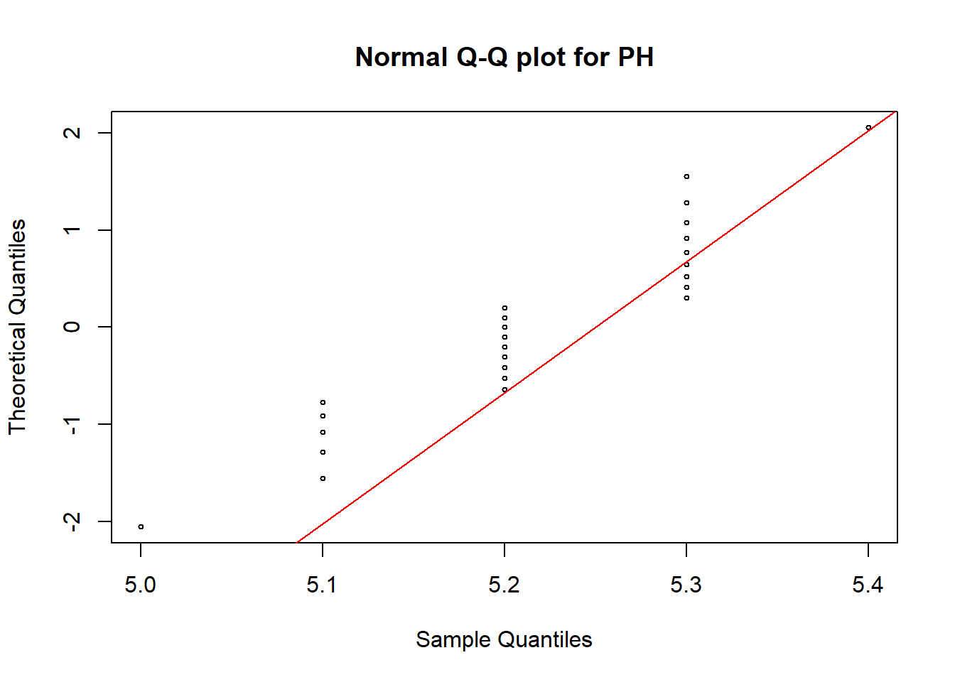

qqnorm(soildata$C, pch = 1, cex = 0.5, datax=T, main="Normal Q-Q plot for C")    
qqline(soildata$C, col = "red", lwd = 1, datax=T)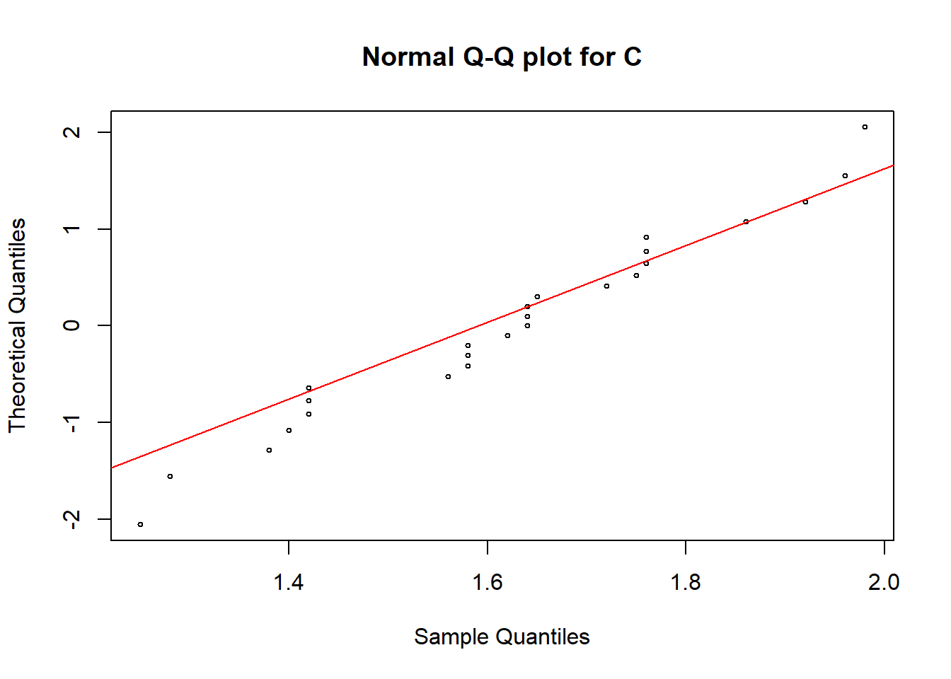

qqnorm(soildata$TN, pch = 1, cex = 0.5, datax=T, main="Normal Q-Q plot for TN")    
qqline(soildata$TN, col = "red", lwd = 1, datax=T)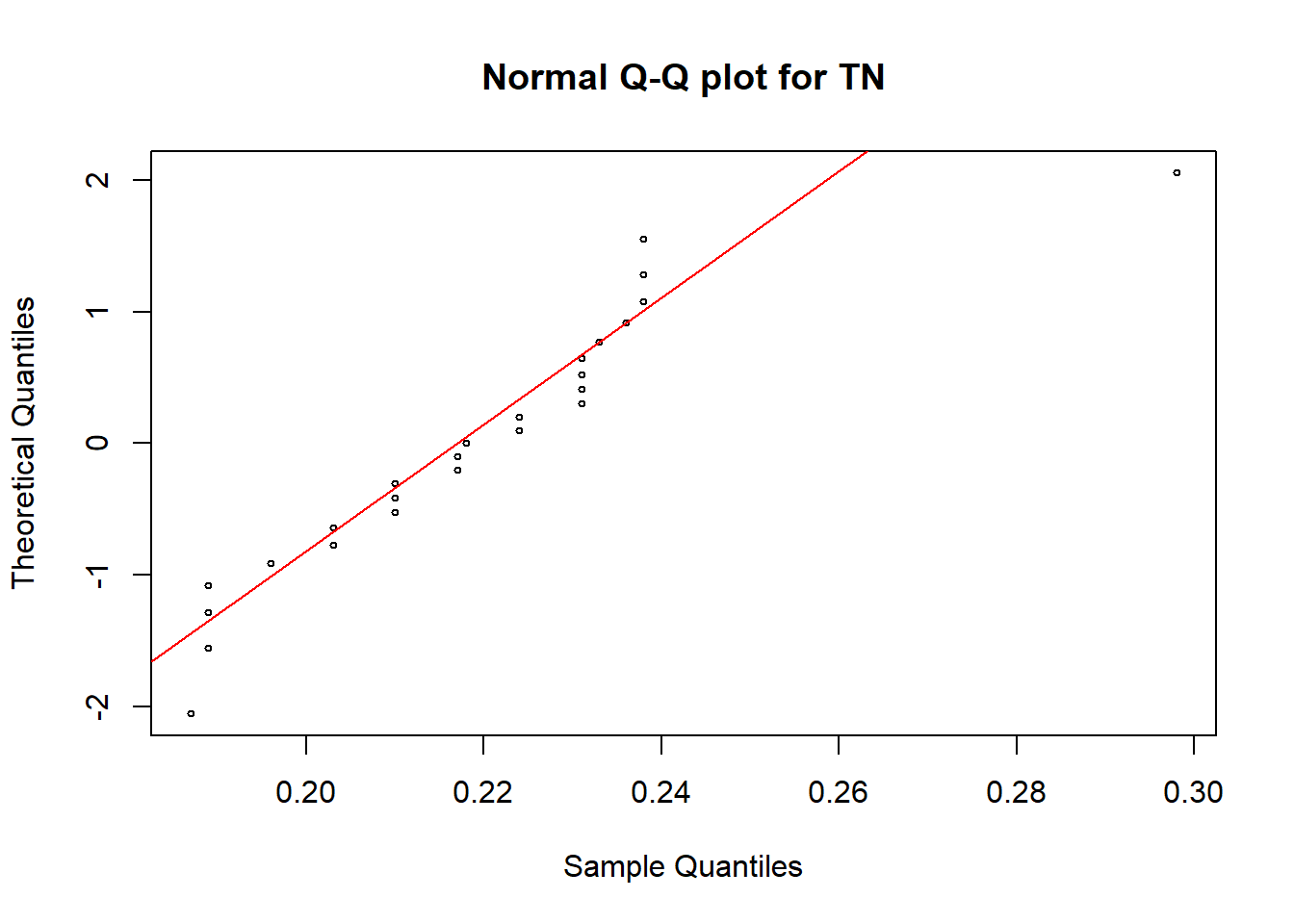

qqnorm(soildata$K, pch = 1, cex = 0.5, datax=T, main="Normal Q-Q plot for K")    
qqline(soildata$K, col = "red", lwd = 1, datax=T)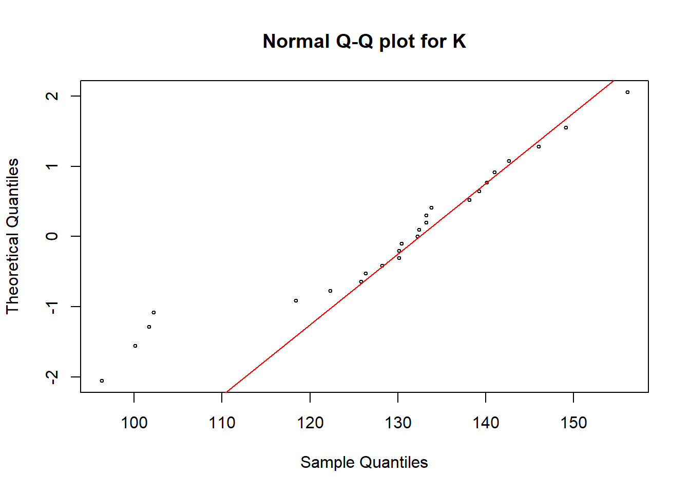

qqnorm(soildata$P, pch = 1, cex = 0.5, datax=T, main="Normal Q-Q plot for P")    
qqline(soildata$P, col = "red", lwd = 1, datax=T)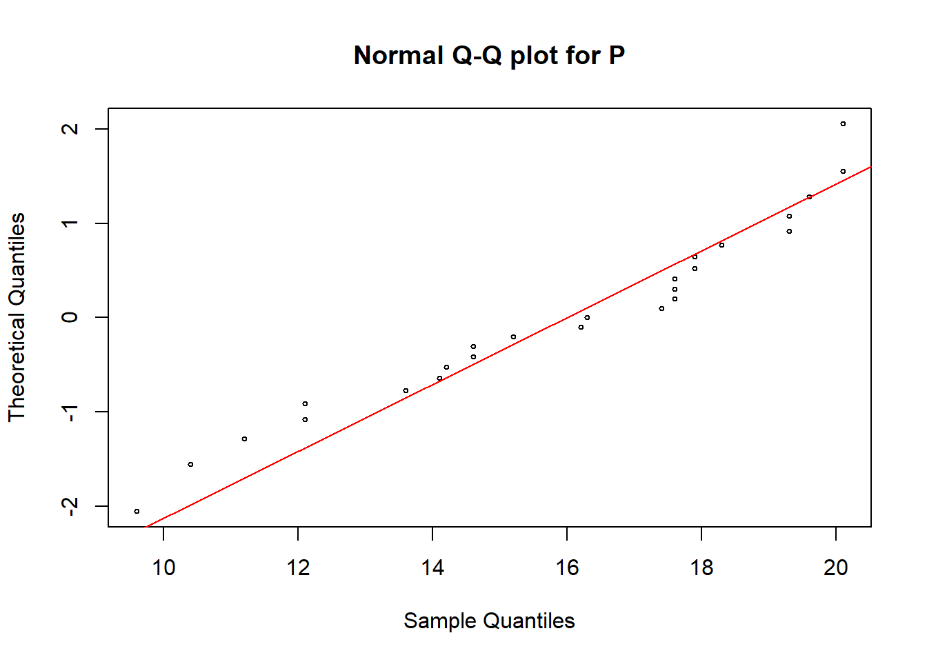

In all these plots we can see some observations are deviated from the straight line. Hence, we need a hypothesis test to make the final conclusion.

Hypothesis tests for testing normality

H0 = data are normally distributed vs H1 = data are not normally distributed

Shapiro–Wilk, Anderson-Darling and Lilliefors tests are three of the tests that can be used to test the above hypothesis. A p-value<0.05 is an evidence that your data were sampled from a non-normal distribution. A p-value>0.05 means that your data are consistent with a Normal distribution.

library(nortest)
# Test each variable
ad.test(soildata$PH)

## 
##  Anderson-Darling normality test
## 
## data:  soildata$PH
## A = 1.2924, p-value = 0.001838

ad.test(soildata$C)

## 
##  Anderson-Darling normality test
## 
## data:  soildata$C
## A = 0.31553, p-value = 0.521

ad.test(soildata$TN)

## 
##  Anderson-Darling normality test
## 
## data:  soildata$TN
## A = 0.71067, p-value = 0.05559

ad.test(soildata$K)

## 
##  Anderson-Darling normality test
## 
## data:  soildata$K
## A = 0.8936, p-value = 0.019

ad.test(soildata$P)

## 
##  Anderson-Darling normality test
## 
## data:  soildata$P
## A = 0.49599, p-value = 0.1942

shapiro.test(soildata$C)

## 
##  Shapiro-Wilk normality test
## 
## data:  soildata$C
## W = 0.96652, p-value = 0.5587

lillie.test(soildata$C)

## 
##  Lilliefors (Kolmogorov-Smirnov) normality test
## 
## data:  soildata$C
## D = 0.12186, p-value = 0.4405

shapiro.test(soildata$P)

## 
##  Shapiro-Wilk normality test
## 
## data:  soildata$P
## W = 0.94018, p-value = 0.1494

lillie.test(soildata$P)

## 
##  Lilliefors (Kolmogorov-Smirnov) normality test
## 
## data:  soildata$P
## D = 0.16754, p-value = 0.06836

According to the Anderson-Darling test, only the soil elements C and P are normally distributed (p>0.05). These results further confirmed by Shapiro–Wilk, and Lilliefors tests.

Single Sample Mean Test

A common and fundamental problem is making inferences about population mean values. Here, we compare population mean with a known value.

Assumptions of Single-sample t-test
• the population variance is unknown
• the underlying distribution is normal or the sample size is at least >30.
• the sample has been randomly selected from the population.

Now we perform a two-sided test separately, to check whether the population mean of C is equal to 1.6, and the population mean of P is equal to 15.5.

mean(soildata$C)

## [1] 1.6212

#H0 = population mean of C is equal to 1.6 vs  H1 = population mean of C is not equal to 1.6 
t.test(soildata$C, alternative = "two.sided", mu = 1.6, conf.level = 0.95)

## 
##  One Sample t-test
## 
## data:  soildata$C
## t = 0.52795, df = 24, p-value = 0.6024
## alternative hypothesis: true mean is not equal to 1.6
## 95 percent confidence interval:
##  1.538324 1.704076
## sample estimates:
## mean of x 
##    1.6212

mean(soildata$P)

## [1] 15.876

#H0 = population mean of P is equal to 15.5 vs  H1 = population mean of P is not equal to 15.5 
t.test(soildata$P, alternative = "two.sided", mu = 15.5, conf.level = 0.95)

## 
##  One Sample t-test
## 
## data:  soildata$P
## t = 0.60311, df = 24, p-value = 0.5521
## alternative hypothesis: true mean is not equal to 15.5
## 95 percent confidence interval:
##  14.58929 17.16271
## sample estimates:
## mean of x 
##    15.876

Note that the sample mean of C is 1.6212, and that of P is 15.876. In both tests, p value > 0.05 which indicates that H0 is not rejected at 5% significance level. Hence, there is a significance evidence that the population mean of C is 1.6 and population mean of P is 15.5. Further, the sample mean is within the respective confidence intervals in both cases which confirms the decision.

Two Sample Variance Tests

Suppose we have two samples selected from two independent populations, and we expect to compare the variances of two populations. In some statistical methods, we need to pool the sample variances before proceeding with a test. Therefore, it is important to test the assumption of homogeneous variances of the two populations.

Assumptions of F-Test
• the underlying distribution is normal or the sample size is at least >30.
• the samples have been randomly and independently selected from two populations

R function
var.test(x, y, ratio = 1,alternative = c("two.sided", "less", "greater"), conf.level = 0.95)

Assume that we have collected soil sample data from two locations. Now we compare the variances of “P” element in these two locations.
H0 = population variance of P in location 1 is equal to the population variance of P in location 2
vs H1 = population variance of P in location 1 is not equal to the population variance of P in location 2

soilP=read.csv("soil-P.csv")
head(soilP)

##   location1 location2
## 1      17.6      14.1
## 2      16.2      19.3
## 3      17.6      14.2
## 4      17.6      13.6
## 5      17.4      14.6
## 6      12.1      20.1

var(soilP$location1)

## [1] 10.8691

var(soilP$location2)

## [1] 8.473333

var.test(soilP$location1,soilP$location2,alternative = "two.sided")

## 
##  F test to compare two variances
## 
## data:  soilP$location1 and soilP$location2
## F = 1.2827, num df = 24, denom df = 24, p-value = 0.5466
## alternative hypothesis: true ratio of variances is not equal to 1
## 95 percent confidence interval:
##  0.5652645 2.9108971
## sample estimates:
## ratio of variances 
##           1.282742

Note that the sample variance of P in location 1 is 10.8691, and that of P in location 2 is 8.473333. Since the p value > 0.05, H0 is not rejected at 5% level of significance. That indicates the population variance of P in location 1 is equal to the population variance of P in location 2 although the sample variances differ.

Two Independent Samples Mean Test

Using this test we can compare the means of two independent populations by taking samples randomly from each population. Examples of two independent populations may include smoking vs. non-smoking, male vs. female, cancer cells vs. normal cells, or treatment A vs. treatment B.

Let us consider the previous example again. i.e. the soil sample data collected from two locations. Suppose we expect to compare the means of “P” element in these two locations.
R function
t.test(x, y = NULL,alternative = c("two.sided", "less", "greater"), mu = 0, paired = FALSE, var.equal = FALSE, conf.level = 0.95)

H0 = population means of P are equal for both locations vs H1 = population means of P are different.

soilP=read.csv("soil-P.csv")
mean(soilP$location1)

## [1] 15.708

mean(soilP$location2)

## [1] 15.68

t.test(soilP$location1,soilP$location2,alternative = "two.sided", conf.level = 0.95) 

## 
##  Welch Two Sample t-test
## 
## data:  soilP$location1 and soilP$location2
## t = 0.031833, df = 47.275, p-value = 0.9747
## alternative hypothesis: true difference in means is not equal to 0
## 95 percent confidence interval:
##  -1.741257  1.797257
## sample estimates:
## mean of x mean of y 
##    15.708    15.680

Sample means of P in location 1 and 2 are 15.708 and 15.68, respectively. Since the p value > 0.05, H0 is not rejected at 5% level of significance. Therefore, the population means of P in two locations are equal.

Two Dependent Samples Mean Tests (Paired sample test)

The paired sample test is used to compare means on the same or related subject over time or in differing circumstances. In a paired experiment, there is a one-to-one correspondence between the values in the two samples (e.g. before and after treatment, or paired subjects).

Example (Darwin Paired Data)
In a classic experiment on plant growth, Charles Darwin took 15 pairs of the plant Zea mays, where the two plants in each pair were “of exactly the same age, were subjected from the first to last to the same conditions, were descended from the same parents”.
One individual was cross-fertilized (CF), the other was self-fertilized (SF). Darwin hypothesized that cross-fertilized plants produced taller offspring than self-fertilized plants.
The heights of the 15 pairs were then measured, and we use this data set to understand the paired sample test.

H0 = cross-fertilized plants do not produce taller offspring than self-fertilized plants
vs H1 = cross-fertilized plants produce taller offspring than self-fertilized plants

paired=read.csv("paireddata.csv")
head(paired)

##   Cross Self
## 1  23.5 17.4
## 2  21.5 20.4
## 3  21.0 20.0
## 4  22.0 20.0
## 5  19.1 18.3
## 6  21.5 18.7

# Testing normality since the sample size is small
ad.test(paired$Cross)

## 
##  Anderson-Darling normality test
## 
## data:  paired$Cross
## A = 0.31949, p-value = 0.5029

ad.test(paired$Self)

## 
##  Anderson-Darling normality test
## 
## data:  paired$Self
## A = 0.33837, p-value = 0.4518

t.test(paired$Cross,paired$Self,paired = TRUE, alternative = "greater", conf.level = 0.95) 

## 
##  Paired t-test
## 
## data:  paired$Cross and paired$Self
## t = 5.4933, df = 14, p-value = 3.958e-05
## alternative hypothesis: true difference in means is greater than 0
## 95 percent confidence interval:
##  2.463863      Inf
## sample estimates:
## mean of the differences 
##                3.626667

Both cross-fertilized and self-fertilized values are normaly distributed. Since the p value < 0.05, for the paired sample test, H0 is rejected at 5% level of significance. Therefore, we can say that Darwin’s hypothesis that cross-fertilized plants produced taller offspring than self-fertilized plants is true at 5% significance level.

Proportion Tests

Proportion tests are used to compare population proportions of two groups of the relevant population/s.

library(MASS)         

## 
## Attaching package: 'MASS'

## The following object is masked from 'package:dplyr':
## 
##     select

head(quine)

##   Eth Sex Age Lrn Days
## 1   A   M  F0  SL    2
## 2   A   M  F0  SL   11
## 3   A   M  F0  SL   14
## 4   A   M  F0  AL    5
## 5   A   M  F0  AL    5
## 6   A   M  F0  AL   13

quine=quine
table(quine$Eth, quine$Sex)

##    
##      F  M
##   A 38 31
##   N 42 35

female.cases=length(which(quine$Eth =="A" & quine$Sex =="F"))
female.cases

## [1] 38

female.total = length(which(quine$Sex=="F"))
female.total

## [1] 80

prop.test(female.cases, female.total, p = 0.5, alternative = "two.sided", conf.level = 0.95, correct = TRUE) 

## 
##  1-sample proportions test with continuity correction
## 
## data:  female.cases out of female.total, null probability 0.5
## X-squared = 0.1125, df = 1, p-value = 0.7373
## alternative hypothesis: true p is not equal to 0.5
## 95 percent confidence interval:
##  0.3633556 0.5890631
## sample estimates:
##     p 
## 0.475

prop.test(table(quine$Eth, quine$Sex), alternative = "two.sided", correct=FALSE) 

## 
##  2-sample test for equality of proportions without continuity
##  correction
## 
## data:  table(quine$Eth, quine$Sex)
## X-squared = 0.0040803, df = 1, p-value = 0.9491
## alternative hypothesis: two.sided
## 95 percent confidence interval:
##  -0.1564218  0.1669620
## sample estimates:
##    prop 1    prop 2 
## 0.5507246 0.5454545