Factor Analysis - Example
To understand the theory and details behind the factor analysis read the Introduction to Factor Analysis.
In this post, an example for factor analysis is given.
Example
Suppose a customer survey was conducted while purchasing car. In the questionnaire, 9 different variables were included, and 75 customers were participated for the study. The survey questions were framed using 5-point likert scale with 1 being very low and 5 being very high. The variables included to the questionnaire were the price, safety, exterior design, space and comfort, technology, resale value, fuel type, color, and maintenance.
Now we import the data set. Suppose your data set is a .csv file named data.csv saved in your working directory. Now, we to import the data using the following codes:
data=read.csv("data.csv")
head(data)
## Price Safety Exterior_Design Space_comfort Technology Resale_Value
## 1 4 4 5 4 3 5
## 2 3 5 3 3 4 3
## 3 4 4 3 4 5 5
## 4 4 4 4 3 3 5
## 5 5 5 4 4 5 5
## 6 4 4 5 3 4 3
## Fuel_Type Color Maintenance
## 1 4 2 4
## 2 4 4 3
## 3 4 4 5
## 4 5 4 4
## 5 3 5 5
## 6 4 2 3Summary statistics
First, we find summary statistics of varibles. We can simply use summary() function to get them. However, here we expect to use stat.desc() function in pastecs package since it gives more descriptive statistics. We apply round function to obtain the resulted values to the second decimal place.
suppressMessages(library(pastecs))
sumstat<- stat.desc(data)
round(sumstat, 2)
## Price Safety Exterior_Design Space_comfort Technology
## nbr.val 75.00 75.00 75.00 75.00 75.00
## nbr.null 0.00 0.00 0.00 0.00 0.00
## nbr.na 0.00 0.00 0.00 0.00 0.00
## min 3.00 3.00 1.00 2.00 1.00
## max 5.00 5.00 5.00 5.00 5.00
## range 2.00 2.00 4.00 3.00 4.00
## sum 314.00 316.00 283.00 297.00 310.00
## median 4.00 4.00 4.00 4.00 4.00
## mean 4.19 4.21 3.77 3.96 4.13
## SE.mean 0.07 0.07 0.10 0.08 0.11
## CI.mean.0.95 0.14 0.15 0.19 0.15 0.21
## var 0.40 0.41 0.69 0.44 0.85
## std.dev 0.63 0.64 0.83 0.67 0.92
## coef.var 0.15 0.15 0.22 0.17 0.22
## Resale_Value Fuel_Type Color Maintenance
## nbr.val 75.00 75.00 75.00 75.00
## nbr.null 0.00 0.00 0.00 0.00
## nbr.na 0.00 0.00 0.00 0.00
## min 1.00 3.00 1.00 2.00
## max 5.00 5.00 5.00 5.00
## range 4.00 2.00 4.00 3.00
## sum 290.00 308.00 279.00 300.00
## median 4.00 4.00 4.00 4.00
## mean 3.87 4.11 3.72 4.00
## SE.mean 0.13 0.08 0.11 0.09
## CI.mean.0.95 0.27 0.16 0.22 0.19
## var 1.33 0.47 0.93 0.65
## std.dev 1.15 0.69 0.97 0.81
## coef.var 0.30 0.17 0.26 0.20Then, we obtain covariances and correlations matrices of the data set. We can either use covariance or correlation matrix to identify factors. Use of correlation matrix indicates that we use standardized variables.
S=cov(data)
S
## Price Safety Exterior_Design Space_comfort
## Price 0.39711712 -0.04036036 0.015855856 0.06162162
## Safety -0.04036036 0.41333333 -0.045585586 0.14378378
## Exterior_Design 0.01585586 -0.04558559 0.691171171 0.07189189
## Space_comfort 0.06162162 0.14378378 0.071891892 0.44432432
## Technology 0.01531532 0.05225225 0.030630631 0.16756757
## Resale_Value 0.29549550 -0.18738739 -0.003603604 -0.14054054
## Fuel_Type 0.06090090 0.08504505 0.038018018 0.22054054
## Color 0.05297297 -0.02054054 -0.280540541 -0.07891892
## Maintenance 0.16216216 -0.12162162 -0.067567568 0.05405405
## Technology Resale_Value Fuel_Type Color
## Price 0.01531532 0.295495495 0.06090090 0.05297297
## Safety 0.05225225 -0.187387387 0.08504505 -0.02054054
## Exterior_Design 0.03063063 -0.003603604 0.03801802 -0.28054054
## Space_comfort 0.16756757 -0.140540541 0.22054054 -0.07891892
## Technology 0.84684685 -0.076576577 0.13423423 0.06486486
## Resale_Value -0.07657658 1.333333333 -0.02612613 0.19189189
## Fuel_Type 0.13423423 -0.026126126 0.47495495 -0.01027027
## Color 0.06486486 0.191891892 -0.01027027 0.93405405
## Maintenance 0.14864865 0.445945946 0.02702703 0.27027027
## Maintenance
## Price 0.16216216
## Safety -0.12162162
## Exterior_Design -0.06756757
## Space_comfort 0.05405405
## Technology 0.14864865
## Resale_Value 0.44594595
## Fuel_Type 0.02702703
## Color 0.27027027
## Maintenance 0.64864865#Total variance
sum(diag(S)) ## [1] 6.183784cor.data=cor(data)
cor.data## Price Safety Exterior_Design Space_comfort
## Price 1.00000000 -0.09961977 0.030264784 0.1466979
## Safety -0.09961977 1.00000000 -0.085287329 0.3355132
## Exterior_Design 0.03026478 -0.08528733 1.000000000 0.1297290
## Space_comfort 0.14669786 0.33551323 0.129728997 1.0000000
## Technology 0.02640974 0.08831864 0.040036923 0.2731728
## Resale_Value 0.40608990 -0.25241826 -0.003753832 -0.1825922
## Fuel_Type 0.14022912 0.19194314 0.066354511 0.4800784
## Color 0.08697792 -0.03305793 -0.349153835 -0.1225025
## Maintenance 0.31951074 -0.23488529 -0.100911513 0.1006870
## Technology Resale_Value Fuel_Type Color
## Price 0.02640974 0.406089905 0.14022912 0.08697792
## Safety 0.08831864 -0.252418262 0.19194314 -0.03305793
## Exterior_Design 0.04003692 -0.003753832 0.06635451 -0.34915384
## Space_comfort 0.27317282 -0.182592194 0.48007841 -0.12250254
## Technology 1.00000000 -0.072064959 0.21165798 0.07293250
## Resale_Value -0.07206496 1.000000000 -0.03283065 0.17194963
## Fuel_Type 0.21165798 -0.032830647 1.00000000 -0.01541948
## Color 0.07293250 0.171949632 -0.01541948 1.00000000
## Maintenance 0.20056436 0.479521510 0.04869309 0.34722222
## Maintenance
## Price 0.31951074
## Safety -0.23488529
## Exterior_Design -0.10091151
## Space_comfort 0.10068702
## Technology 0.20056436
## Resale_Value 0.47952151
## Fuel_Type 0.04869309
## Color 0.34722222
## Maintenance 1.00000000To visualize these correlations, now we obtain the correlation plot by using corrplot package.
suppressMessages(library(corrplot))
corrplot(cor.data, order = "AOE", method = "circle", bg = "grey", tl.cex=0.8, col = colorRampPalette(c("yellow","green","navyblue"))(100))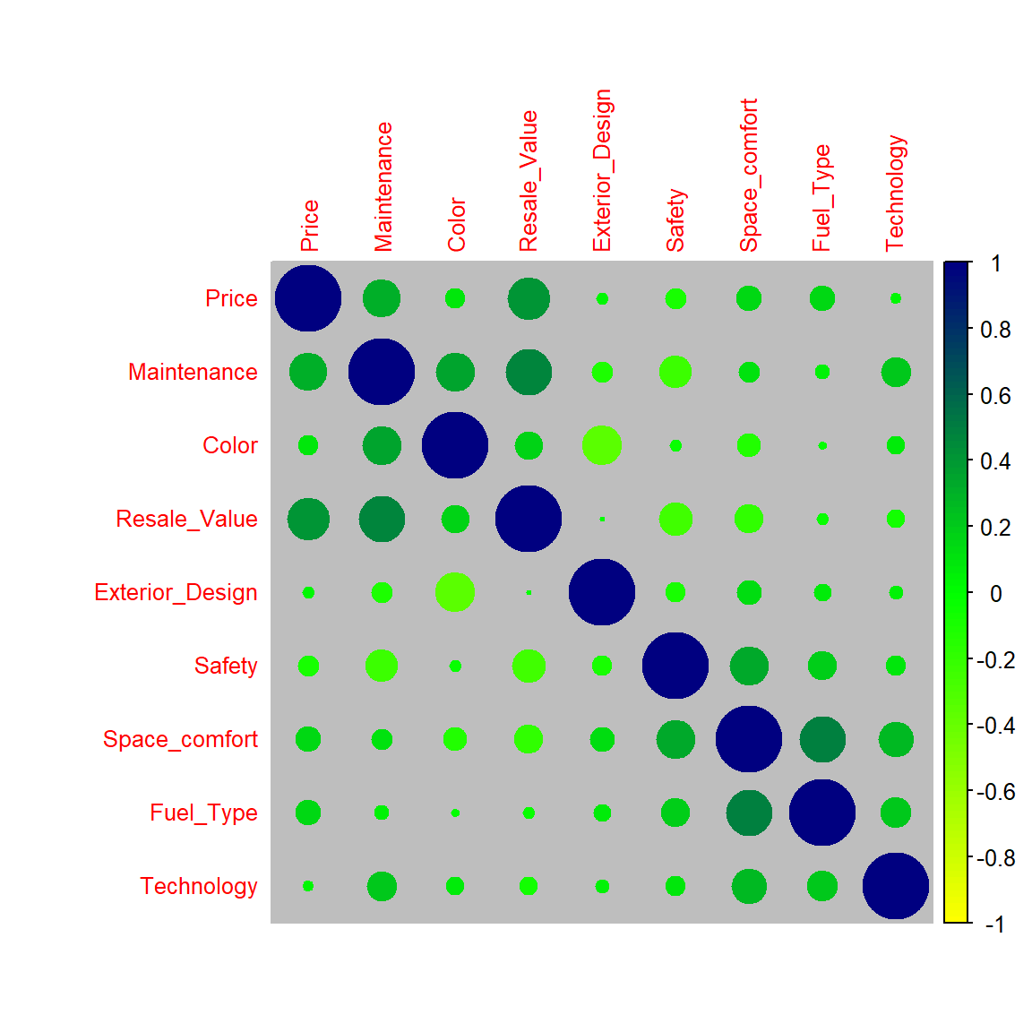
In this plot, positive correlations are displayed in blue and negative correlations in red color. Color intensity and the size of the circles are proportional to the correlation coefficients. The correlation plot shows that most of the variables are fairly correlated.
Correlation tests
Now, we apply Bartlett’s test of sphericity (the null hypothesis of the test is that there is no correlation between the variables) to identify whether the above correlations are significant. The test statistic follows a chi square distribution.
suppressMessages(library(REdaS))
bart_spher(data)
## Bartlett's Test of Sphericity
##
## Call: bart_spher(x = data)
##
## X2 = 110.805
## df = 36
## p-value < 2.22e-16According to the Bartlett’s test of sphericity results, there is a significant (p < 0.000) correlation among variables. This indicates that factor analysis can be performed and the variables can be grouped.
Testing the assumptions to do factor analysis, KMO test is used which measures Sampling Accuracy(MSA). The overall MSA value has to be greater than 0.5 from KMO test to do factor analysis.
library(psych)
data.KMO <- KMO(cor.data)
data.KMO
## Kaiser-Meyer-Olkin factor adequacy
## Call: KMO(r = cor.data)
## Overall MSA = 0.58
## MSA for each item =
## Price Safety Exterior_Design Space_comfort
## 0.67 0.60 0.53 0.52
## Technology Resale_Value Fuel_Type Color
## 0.65 0.58 0.64 0.58
## Maintenance
## 0.56Here the overall MSA=0.58 which is greater than 0.5, and we can perform factor analysis.
Extracting factors
We use the correlation matrix for eigen analysis.
R.eigen <- eigen(cor(data))
R.eigen
## eigen() decomposition
## $values
## [1] 2.0991580 1.8826227 1.3426882 0.9493682 0.6852855 0.6128772 0.5617019
## [8] 0.5521248 0.3141736
##
## $vectors
## [,1] [,2] [,3] [,4] [,5]
## [1,] 0.35208657 -0.29959115 0.26223876 -0.40688984 0.25290772
## [2,] -0.35104767 -0.23797874 -0.32525215 -0.38787589 0.58564776
## [3,] -0.15889801 -0.07501709 0.67225367 0.24010197 0.09309004
## [4,] -0.22084213 -0.57248368 0.03323658 -0.08809602 -0.02650783
## [5,] -0.02342334 -0.40184482 -0.13248698 0.71305186 0.31788215
## [6,] 0.52939758 -0.05999686 0.22690195 -0.19187880 0.16172774
## [7,] -0.12536500 -0.52480053 0.01805726 -0.16813505 -0.65848265
## [8,] 0.35617344 -0.05608604 -0.54939200 0.05411791 -0.14736644
## [9,] 0.50536562 -0.27677794 -0.03488957 0.20524260 0.03412889
## [,6] [,7] [,8] [,9]
## [1,] 0.431400452 -0.50119993 0.1636832 0.15456214
## [2,] -0.342595309 0.05087181 -0.2016247 0.24555996
## [3,] -0.583047558 -0.30690187 0.1010309 0.08089313
## [4,] 0.004657572 0.26643126 0.5055957 -0.53599311
## [5,] 0.268603616 -0.16486300 -0.3227215 -0.08631563
## [6,] -0.220083482 0.26172032 -0.5122925 -0.47149003
## [7,] -0.054034721 -0.07776970 -0.4310997 0.22772426
## [8,] -0.450906799 -0.51300094 0.1858511 -0.20613131
## [9,] -0.172437302 0.46490956 0.2823838 0.54578095fit <- princomp(data, cor=TRUE)
plot(fit,type="lines") # scree plot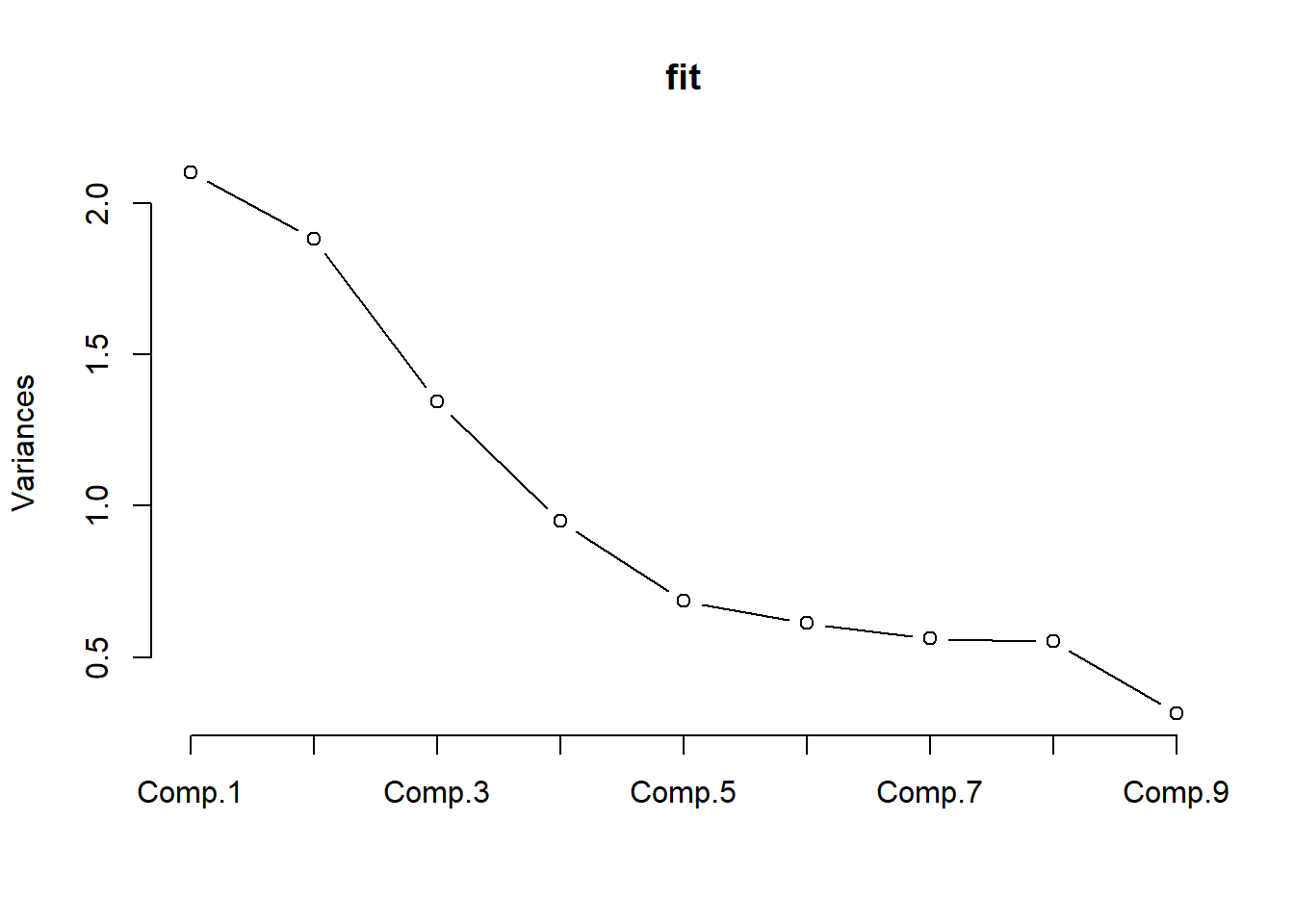
Here we check the number of eigen values greater than or equal to 0.7, which is the Jolliffe’s method for identifying number of principal components. Here we have four eigen values greater than 0.7. The non-steep of the graph, which is called scree plot, can be seen after the fourth eigen value. That implies we can have four hidden common factors corresponding to the data. Now we obtain factor loadings, proportion of variance and the biplot.
fit <- princomp(data, cor=TRUE)
summary(fit) # print variance accounted for
## Importance of components:
## Comp.1 Comp.2 Comp.3 Comp.4 Comp.5
## Standard deviation 1.4488471 1.3720870 1.1587442 0.9743553 0.82781974
## Proportion of Variance 0.2332398 0.2091803 0.1491876 0.1054854 0.07614284
## Cumulative Proportion 0.2332398 0.4424201 0.5916076 0.6970930 0.77323584
## Comp.6 Comp.7 Comp.8 Comp.9
## Standard deviation 0.78286472 0.74946772 0.7430510 0.56051192
## Proportion of Variance 0.06809746 0.06241132 0.0613472 0.03490818
## Cumulative Proportion 0.84133330 0.90374462 0.9650918 1.00000000loadings(fit) # pc loadings ##
## Loadings:
## Comp.1 Comp.2 Comp.3 Comp.4 Comp.5 Comp.6 Comp.7 Comp.8
## Price 0.352 0.300 0.262 0.407 0.253 0.431 0.501 0.164
## Safety -0.351 0.238 -0.325 0.388 0.586 -0.343 -0.202
## Exterior_Design -0.159 0.672 -0.240 -0.583 0.307 0.101
## Space_comfort -0.221 0.572 -0.266 0.506
## Technology 0.402 -0.132 -0.713 0.318 0.269 0.165 -0.323
## Resale_Value 0.529 0.227 0.192 0.162 -0.220 -0.262 -0.512
## Fuel_Type -0.125 0.525 0.168 -0.658 -0.431
## Color 0.356 -0.549 -0.147 -0.451 0.513 0.186
## Maintenance 0.505 0.277 -0.205 -0.172 -0.465 0.282
## Comp.9
## Price 0.155
## Safety 0.246
## Exterior_Design
## Space_comfort -0.536
## Technology
## Resale_Value -0.471
## Fuel_Type 0.228
## Color -0.206
## Maintenance 0.546
##
## Comp.1 Comp.2 Comp.3 Comp.4 Comp.5 Comp.6 Comp.7 Comp.8
## SS loadings 1.000 1.000 1.000 1.000 1.000 1.000 1.000 1.000
## Proportion Var 0.111 0.111 0.111 0.111 0.111 0.111 0.111 0.111
## Cumulative Var 0.111 0.222 0.333 0.444 0.556 0.667 0.778 0.889
## Comp.9
## SS loadings 1.000
## Proportion Var 0.111
## Cumulative Var 1.000fit$scores # the principal components## Comp.1 Comp.2 Comp.3 Comp.4 Comp.5
## [1,] -0.3035647 -0.64402922 2.401017368 0.54219661 -0.002072474
## [2,] -1.5357999 -1.69042873 -1.847094738 -0.02285481 0.041620717
## [3,] 1.4037520 0.51633338 -0.705154680 -0.80574458 0.203640827
## [4,] 0.7812858 -0.71602472 0.418573635 0.83275816 -1.343683825
## [5,] 1.7782536 0.75023698 -0.580130769 -0.14107251 2.445867595
## [6,] -1.5504758 -1.51963095 1.853840625 -0.44895365 0.061053399
## [7,] -1.2940078 -1.63806818 -1.142645305 0.28289125 -1.263240227
## [8,] 1.7610426 0.23452307 0.618215901 -1.70386881 -0.600699841
## [9,] 1.0009405 -0.04857035 1.675391215 1.07947933 0.094947781
## [10,] 1.9251728 0.47675597 -1.301257466 -0.74955884 -0.871737542
## [11,] 1.5176545 -0.11765081 -0.268980126 -0.14477340 1.526919964
## [12,] 2.4655956 -0.57167906 -0.004264804 -1.89329350 -0.714171625
## [13,] 0.3281424 -0.29805680 2.357405401 0.28564336 0.040588637
## [14,] 0.2327117 0.97543083 -1.719850741 0.31725795 1.046566607
## [15,] 2.1202064 -1.06971520 0.712957619 -1.05685090 -0.908423998
## [16,] 1.5736536 0.59479523 -0.498629430 1.85021420 -1.245918065
## [17,] 0.6780655 -0.71590939 1.372030770 -0.44928822 1.237528021
## [18,] 0.4806337 0.41171598 -1.100806921 -1.14032643 -0.078366187
## [19,] 2.1210760 0.56139556 -1.418007843 0.26223468 1.411269652
## [20,] 1.4293769 0.07672020 -0.560215587 -0.02567480 -0.144118250
## [21,] 1.5906813 1.85241211 0.554221362 -0.20085440 -0.241505817
## [22,] 2.2094365 -1.77511726 -0.801088373 -1.59160206 0.092347571
## [23,] 1.4037520 0.51633338 -0.705154680 -0.80574458 0.203640827
## [24,] 1.3345222 0.64897391 -0.242602207 0.10083704 0.565013378
## [25,] 1.0538289 0.93418597 0.280219950 -0.07081300 -0.993298557
## [26,] 3.0700391 -1.64807614 1.492233587 -0.21948465 0.068976748
## [27,] -1.2376319 -0.47983122 -1.840509329 -0.14635618 0.044246908
## [28,] 0.4806337 0.41171598 -1.100806921 -1.14032643 -0.078366187
## [29,] 1.2934657 0.13078355 -1.257645499 -0.49300559 -0.914398653
## [30,] 2.5322769 -0.49310188 1.155717581 -0.51938110 0.417481330
## [31,] -0.3035647 -0.64402922 2.401017368 0.54219661 -0.002072474
## [32,] 0.1787338 0.23603967 -0.563364110 1.74483565 1.091660136
## [33,] -2.1498078 -0.89034086 -0.454504583 0.39023364 0.449602711
## [34,] -1.3117294 1.94066453 3.222550278 0.32367380 0.206383430
## [35,] 0.2012052 -1.49543259 0.283849069 0.22521592 1.998462073
## [36,] 1.5302949 0.50302445 -0.339101202 0.45706264 0.118911906
## [37,] 2.2173047 1.72309056 -0.369444440 0.68638891 -1.771819318
## [38,] -1.8583900 -1.09461904 2.048977094 0.46416800 -0.326740599
## [39,] -0.3968574 -4.44702999 0.108183041 1.68149221 0.086859885
## [40,] -1.9690735 -2.07581138 -0.939505109 -0.85370707 0.058928633
## [41,] -0.5891435 0.90855621 -0.383307167 0.62582492 -0.259896229
## [42,] -0.7389407 -2.85766686 -1.164653964 1.94170267 0.712042811
## [43,] -0.5516685 1.83160426 -0.905393120 0.70250397 -0.453437854
## [44,] -0.9483073 2.21279448 -0.478048884 -0.02119298 0.047827927
## [45,] -2.7677848 -0.85900317 -0.242329057 0.97133755 0.042086352
## [46,] 0.1436950 -0.23071987 0.099627878 -0.22716111 -0.215056590
## [47,] 0.8860344 3.23895257 0.336880063 0.19245161 0.594745782
## [48,] -0.1603567 -0.61004012 -0.269515255 -1.42013226 0.953605565
## [49,] -0.9495711 -0.62900099 -0.054586275 -0.13789879 -0.398721208
## [50,] -0.4924520 -0.24114189 1.251214057 -0.27600020 -1.983184529
## [51,] -1.2561896 -1.69519880 -0.544384060 -0.09112014 -0.458909368
## [52,] -0.7794232 -0.33533727 -0.296024363 -0.56174297 -0.497063603
## [53,] 1.7581964 1.11713564 -2.339594033 4.47572524 -1.247195639
## [54,] -1.1407230 2.30363553 0.336008733 -0.31194162 0.160554205
## [55,] 1.6406672 -1.86860973 1.267562158 1.24257934 -1.383573107
## [56,] -0.8462550 0.21614906 0.625150716 1.34316892 1.216889612
## [57,] -0.8590260 -0.63511525 0.715523175 0.08576496 -0.104210997
## [58,] 0.3268273 -0.99734460 0.073249959 -0.47277155 0.746849995
## [59,] -2.7964664 1.42674146 -0.237145925 -0.87270766 -0.427144076
## [60,] -0.1565597 1.49266334 1.016238706 -0.56963164 -0.453447663
## [61,] -1.8798760 2.25257679 -1.356913502 -0.43249756 -0.291741056
## [62,] 0.3351582 0.18947012 1.090851712 0.47924008 0.342483777
## [63,] -1.0595808 2.95295203 2.428187258 0.25065198 1.067769092
## [64,] -0.3887173 -1.48449642 -1.282347745 0.20827263 0.758617497
## [65,] -1.8501103 2.23470336 0.358960797 0.77447053 0.421703676
## [66,] -1.8501103 2.23470336 0.358960797 0.77447053 0.421703676
## [67,] -2.0873794 -0.29534941 -1.127778838 -0.96062135 0.462071152
## [68,] -1.1129623 0.52928782 -0.245826987 -0.42869109 -0.537098524
## [69,] -1.7821443 -0.73973265 0.319870933 -0.24881690 -0.386218011
## [70,] -0.1136409 -0.57337774 0.288515140 0.03849628 -0.744599600
## [71,] -1.1385871 0.96890100 -0.390766081 -1.20876087 -0.189339447
## [72,] -0.3434890 0.15658461 -0.243137336 -1.17452182 -0.008301020
## [73,] -0.5083638 0.34755386 -2.380565535 0.01435104 0.683313370
## [74,] -3.0149377 -0.06441640 -0.415456867 -1.60059553 -1.545402689
## [75,] 0.2893523 -1.92039265 0.595335912 -0.54945060 0.940391620
## Comp.6 Comp.7 Comp.8 Comp.9
## [1,] -0.6141886842 -1.08694448 -0.17272212 -0.06537187
## [2,] -0.4810407951 -0.02157190 -1.18377885 0.30187907
## [3,] 0.2306425558 -0.98189173 -0.38334346 -0.19735549
## [4,] -0.9335111884 0.12616621 -1.30122559 0.54940243
## [5,] -0.7134383005 0.53155158 0.50810910 -0.01533283
## [6,] 0.2719353454 0.53330859 -0.74906706 0.78963097
## [7,] -0.2313847683 -0.52466221 0.24860280 -0.79772871
## [8,] 0.0610786738 -0.53059228 0.05472322 -0.48392172
## [9,] -0.8643924552 0.78250128 0.47596043 -0.24789078
## [10,] -0.3250199011 0.06848217 -1.58309967 0.73009550
## [11,] 1.2143080960 0.28633362 0.15491677 -0.96531828
## [12,] -0.4156502630 0.40617622 -0.51528574 0.11087135
## [13,] -0.8297353110 -1.66808142 0.18025764 0.61685432
## [14,] 0.5129721176 1.31102027 0.29633188 0.35928638
## [15,] -0.2398046616 -0.30855781 -0.35582737 0.42001969
## [16,] -0.0009514879 0.68720428 -0.20487626 -0.32586613
## [17,] 0.2490817246 -1.97296795 0.33460943 0.09181162
## [18,] 0.6144053324 -0.52552619 0.50994850 0.62478856
## [19,] -0.0933716406 0.67591031 -1.00758419 1.02888171
## [20,] -0.0632064249 -1.16224979 -0.03029018 -0.10292727
## [21,] 0.1348598939 0.30404666 -0.62925579 0.48018032
## [22,] 0.5848644189 0.50206858 -0.36086043 -1.00196933
## [23,] 0.2306425558 -0.98189173 -0.38334346 -0.19735549
## [24,] 1.1353745758 0.39993902 -0.47483048 -0.63266036
## [25,] -0.8481744799 -0.67700520 -0.53769525 0.32768722
## [26,] -0.9412638458 1.10418770 1.20440298 0.31194776
## [27,] -0.6895530673 -1.00510136 -0.06719523 0.17459207
## [28,] 0.6144053324 -0.52552619 0.50994850 0.62478856
## [29,] -0.1094732743 0.64961911 -1.93607942 0.04786931
## [30,] 0.5353486064 -0.02386194 1.29901648 -0.47523010
## [31,] -0.6141886842 -1.08694448 -0.17272212 -0.06537187
## [32,] 0.5206015692 0.72105765 -0.79048146 -0.83593553
## [33,] 0.2735013354 -1.72089914 -1.25401077 -0.48926591
## [34,] 1.2760367137 -0.16756072 -1.03005397 -0.95166832
## [35,] -0.5485712379 -0.53472277 -0.90410380 0.38890131
## [36,] 0.8178603565 -0.13337322 0.67784853 0.55506607
## [37,] 1.7965849902 -0.94232204 0.55844151 -0.81534061
## [38,] -0.0148792807 -0.04944199 0.36759009 0.07454599
## [39,] 0.7221762757 0.60543138 -1.02753231 -0.04858881
## [40,] 0.8029737029 -0.76410276 0.77834784 -0.59902270
## [41,] -0.9772171175 0.05265425 -0.75975353 0.44105585
## [42,] -0.3006198431 0.30480040 0.41356769 0.40499890
## [43,] -1.4398773449 0.18463771 0.19744524 -0.58317746
## [44,] -0.6763337822 -0.16938021 -0.34920294 -0.46288555
## [45,] 0.0687527959 0.49000007 1.01641026 0.96853615
## [46,] -0.3618129445 0.01870912 0.18571822 -0.27612487
## [47,] -1.5703055211 0.72800904 0.13456066 -0.06157361
## [48,] 0.2028509447 0.31364454 0.90905816 -0.29213898
## [49,] 0.0456150707 0.82802883 0.27938444 -0.54727904
## [50,] 0.7809653970 0.25873574 -0.67487918 -0.79549583
## [51,] 1.4061912212 0.55258896 -0.35351053 0.79006973
## [52,] 0.0219498321 0.47507465 1.07901017 0.54601918
## [53,] 0.0784366953 -1.47997993 1.05740505 -0.07568704
## [54,] -1.3823683170 0.20225897 -0.22686076 -0.36492898
## [55,] 0.2691107854 0.94073959 0.70543815 0.58464327
## [56,] 0.4761430048 0.78650362 -0.41508821 -0.11218682
## [57,] 0.3234282644 0.06547008 -0.36085644 -0.74363094
## [58,] -0.2828794243 -0.09489628 0.81546546 -0.60878279
## [59,] -1.6641256949 0.21088489 -0.39468728 -0.88300447
## [60,] 0.0281347626 1.71318833 0.03339859 0.71805475
## [61,] 0.8594928727 -0.97198402 1.02777766 1.56932025
## [62,] 0.7970670307 0.28502694 0.25361605 0.18551657
## [63,] 0.5003541955 -1.18131211 -0.19317299 1.20837889
## [64,] -2.2720790330 -0.62123242 0.78489640 -0.59147320
## [65,] 0.8899742082 0.90625732 -0.18763889 -0.27239828
## [66,] 0.8899742082 0.90625732 -0.18763889 -0.27239828
## [67,] -0.8861919945 0.12803282 -0.65088608 -0.50410577
## [68,] 0.0289841867 0.07268213 1.84261404 -0.26349402
## [69,] 0.7071910410 0.52183562 0.53243551 0.07851311
## [70,] -1.6395096538 0.97254899 1.30135456 0.11261182
## [71,] 0.3228331674 0.25304018 1.48956077 -0.35792223
## [72,] 0.1239174245 0.42724994 0.27931092 0.04051894
## [73,] 0.9995158413 -0.39568870 -0.28109794 0.22912860
## [74,] 0.4248024967 0.24328804 -0.26521176 0.48089351
## [75,] 0.1797808031 -0.22687974 -0.14173331 0.41545053biplot(fit,scale=0)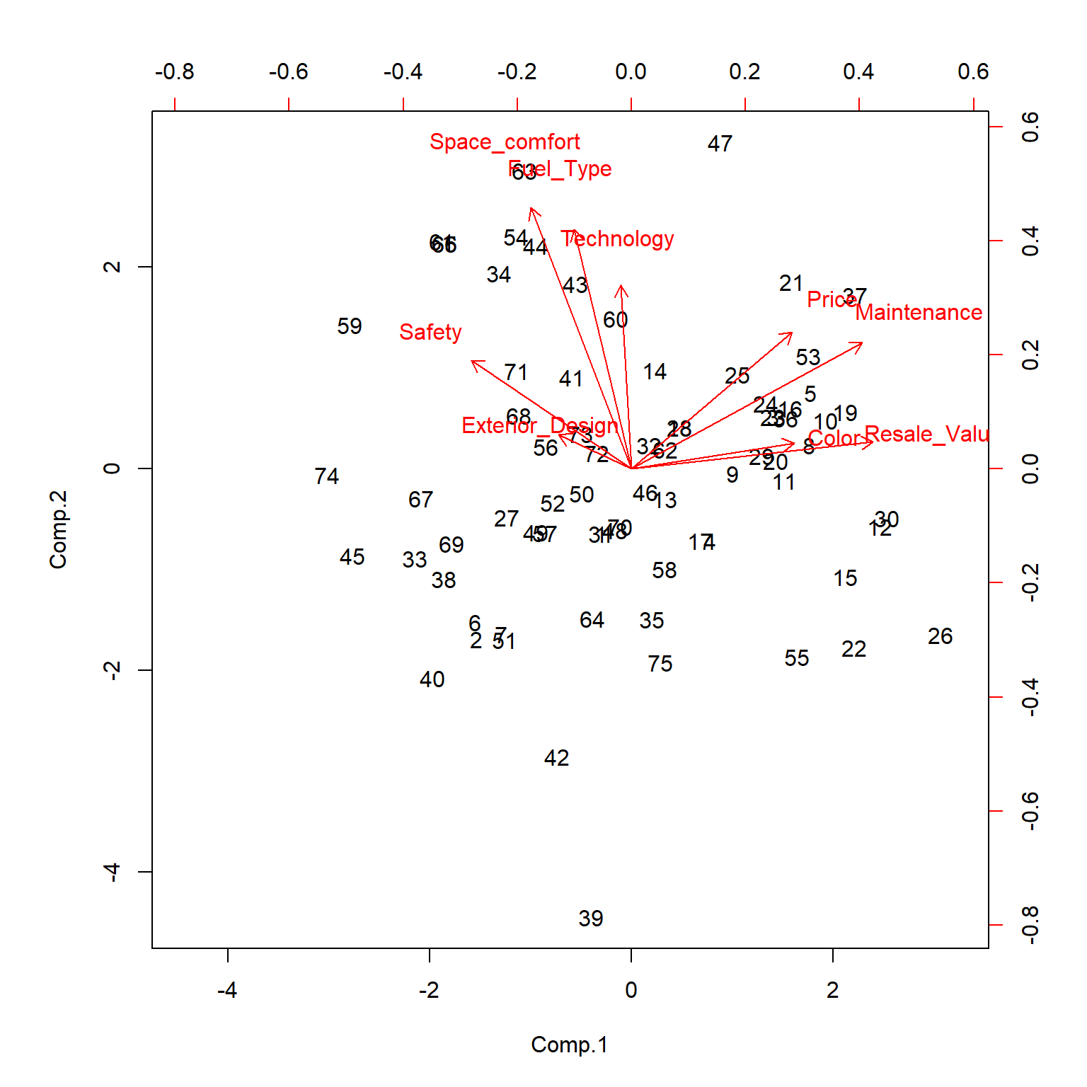
Note that the cumulative proportion of variance of the first four principal components explains approximately 70% of the variance of the data. Facator loadings for all 9 components are shown, and they are correlated.Biplot clealy shows the four different facors visually.
Parallel Analysis
To confirn the number of factors further, we now perform Parallel Analysis. The function fa.parallel function in psych package can be used to execute parallel analysis. Here we apply minres as the factor method, and identify the acceptable number of factors by generating the scree plot.
suppressMessages(library(psych))
fa.parallel(data, fm = 'minres', fa = 'fa')
## The estimated weights for the factor scores are probably incorrect. Try a different factor extraction method.
## The estimated weights for the factor scores are probably incorrect. Try a different factor extraction method.
## The estimated weights for the factor scores are probably incorrect. Try a different factor extraction method.
## The estimated weights for the factor scores are probably incorrect. Try a different factor extraction method.
## The estimated weights for the factor scores are probably incorrect. Try a different factor extraction method.
## The estimated weights for the factor scores are probably incorrect. Try a different factor extraction method.
## The estimated weights for the factor scores are probably incorrect. Try a different factor extraction method.
## The estimated weights for the factor scores are probably incorrect. Try a different factor extraction method.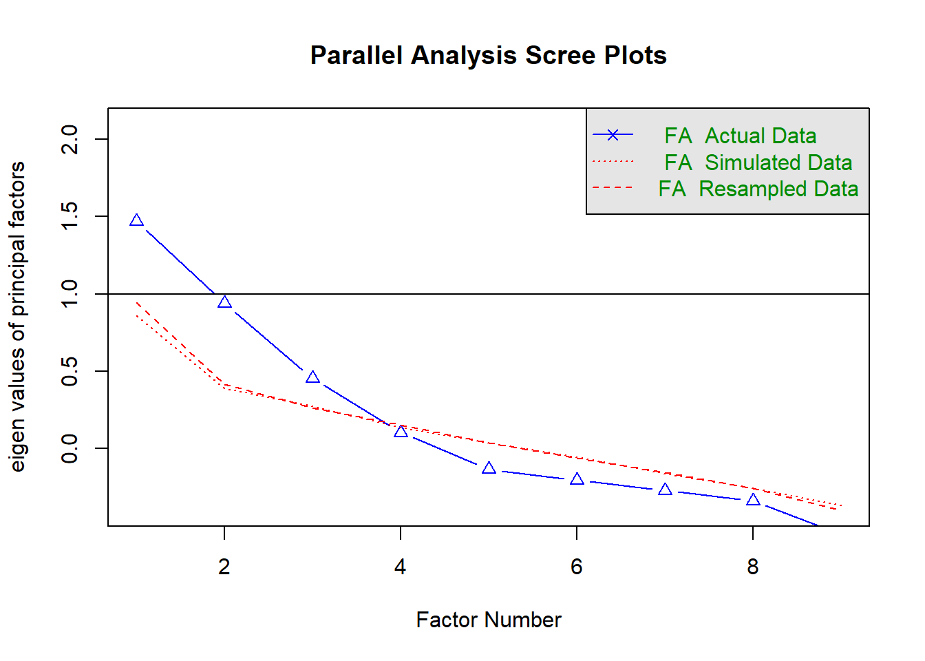
## Parallel analysis suggests that the number of factors = 3 and the number of components = NAThe output suggests the maximum number of factors is 3. But it is also closer to 4. The blue line of the scree plot shows eigenvalues of actual data and the two red lines show simulated and resampled data. Here, we have to check the large steep in the actual data and identify the point where it levels off to the right. Also, we have to locate the the point where the gap between simulated data and actual data tends to be minimum. Therefore, the parallel analysis scree plot suggests that anywhere between 3 to 4 factors would be a good choice.
Factor rotation
If the original loadings are not clear, and may not be readily interpretable, it is usual practice to rotate them until a simple structure is achieved. The fa( ) function in psych package can be used to rotate factors. If the factors are uncorrelated we can use varimax factor rotation, and otherwise we use Oblimin factor rotation. As the factor extraction method, we apply Minimum Residual (OLS). The other available methods are Maximum Liklihood, Principal Component etc.
Since the original factors are correlated, we apply oblique rotation (oblimin). Also, we use Ordinary Least Squared factoring i.e. minres for the argument fm in fa( ) function. This factoring method provides results similar to Maximum Likelihood method without assuming multivariate normal distribution, and derives solutions through iterative eigen analysis. First, we start by considering a three factor model.
suppressMessages(library(GPArotation))
obli3factor <- fa(data,nfactors = 3,rotate = "oblimin",fm="minres")
print(obli3factor)
## Factor Analysis using method = minres
## Call: fa(r = data, nfactors = 3, rotate = "oblimin", fm = "minres")
## Standardized loadings (pattern matrix) based upon correlation matrix
## MR2 MR1 MR3 h2 u2 com
## Price 0.18 0.53 -0.06 0.29 0.71 1.3
## Safety 0.34 -0.37 0.14 0.25 0.75 2.3
## Exterior_Design 0.10 0.15 -0.51 0.25 0.75 1.2
## Space_comfort 0.91 -0.01 -0.05 0.83 0.17 1.0
## Technology 0.34 0.03 0.12 0.13 0.87 1.3
## Resale_Value -0.14 0.75 -0.05 0.57 0.43 1.1
## Fuel_Type 0.54 0.05 0.00 0.30 0.70 1.0
## Color -0.04 0.07 0.72 0.56 0.44 1.0
## Maintenance 0.15 0.63 0.26 0.57 0.43 1.4
##
## MR2 MR1 MR3
## SS loadings 1.43 1.42 0.90
## Proportion Var 0.16 0.16 0.10
## Cumulative Var 0.16 0.32 0.42
## Proportion Explained 0.38 0.38 0.24
## Cumulative Proportion 0.38 0.76 1.00
##
## With factor correlations of
## MR2 MR1 MR3
## MR2 1.00 -0.04 -0.06
## MR1 -0.04 1.00 0.27
## MR3 -0.06 0.27 1.00
##
## Mean item complexity = 1.3
## Test of the hypothesis that 3 factors are sufficient.
##
## The degrees of freedom for the null model are 36 and the objective function was 1.58 with Chi Square of 110.8
## The degrees of freedom for the model are 12 and the objective function was 0.12
##
## The root mean square of the residuals (RMSR) is 0.03
## The df corrected root mean square of the residuals is 0.06
##
## The harmonic number of observations is 75 with the empirical chi square 6.43 with prob < 0.89
## The total number of observations was 75 with Likelihood Chi Square = 8.05 with prob < 0.78
##
## Tucker Lewis Index of factoring reliability = 1.165
## RMSEA index = 0 and the 90 % confidence intervals are 0 0.08
## BIC = -43.76
## Fit based upon off diagonal values = 0.97
## Measures of factor score adequacy
## MR2 MR1 MR3
## Correlation of (regression) scores with factors 0.92 0.86 0.80
## Multiple R square of scores with factors 0.85 0.75 0.65
## Minimum correlation of possible factor scores 0.70 0.49 0.29Since there is a loading for each variable on all three factors, we consider the loadings more than 0.3 as the cutoff value for not getting loading on more than one factor.
print(obli3factor$loadings,cutoff = 0.3)##
## Loadings:
## MR2 MR1 MR3
## Price 0.531
## Safety 0.340 -0.370
## Exterior_Design -0.510
## Space_comfort 0.906
## Technology 0.345
## Resale_Value 0.748
## Fuel_Type 0.544
## Color 0.722
## Maintenance 0.633
##
## MR2 MR1 MR3
## SS loadings 1.435 1.409 0.890
## Proportion Var 0.159 0.157 0.099
## Cumulative Var 0.159 0.316 0.415Since the variable safety is loaded on two factors, we will consider the four factor model.
obli4factor <- fa(data,nfactors = 4,rotate = "oblimin",fm="minres")
print(obli4factor$loadings,cutoff = 0.3)
##
## Loadings:
## MR2 MR1 MR4 MR3
## Price 0.602
## Safety 0.423
## Exterior_Design -0.671
## Space_comfort 0.868
## Technology 0.338
## Resale_Value 0.694
## Fuel_Type 0.571
## Color 0.476
## Maintenance 0.896
##
## MR2 MR1 MR4 MR3
## SS loadings 1.408 1.085 0.918 0.736
## Proportion Var 0.156 0.121 0.102 0.082
## Cumulative Var 0.156 0.277 0.379 0.461Factor mapping
Now, the variables have only single-loading,and we have a simple structure. Then, we look at the factor mapping.
fa.diagram(obli4factor)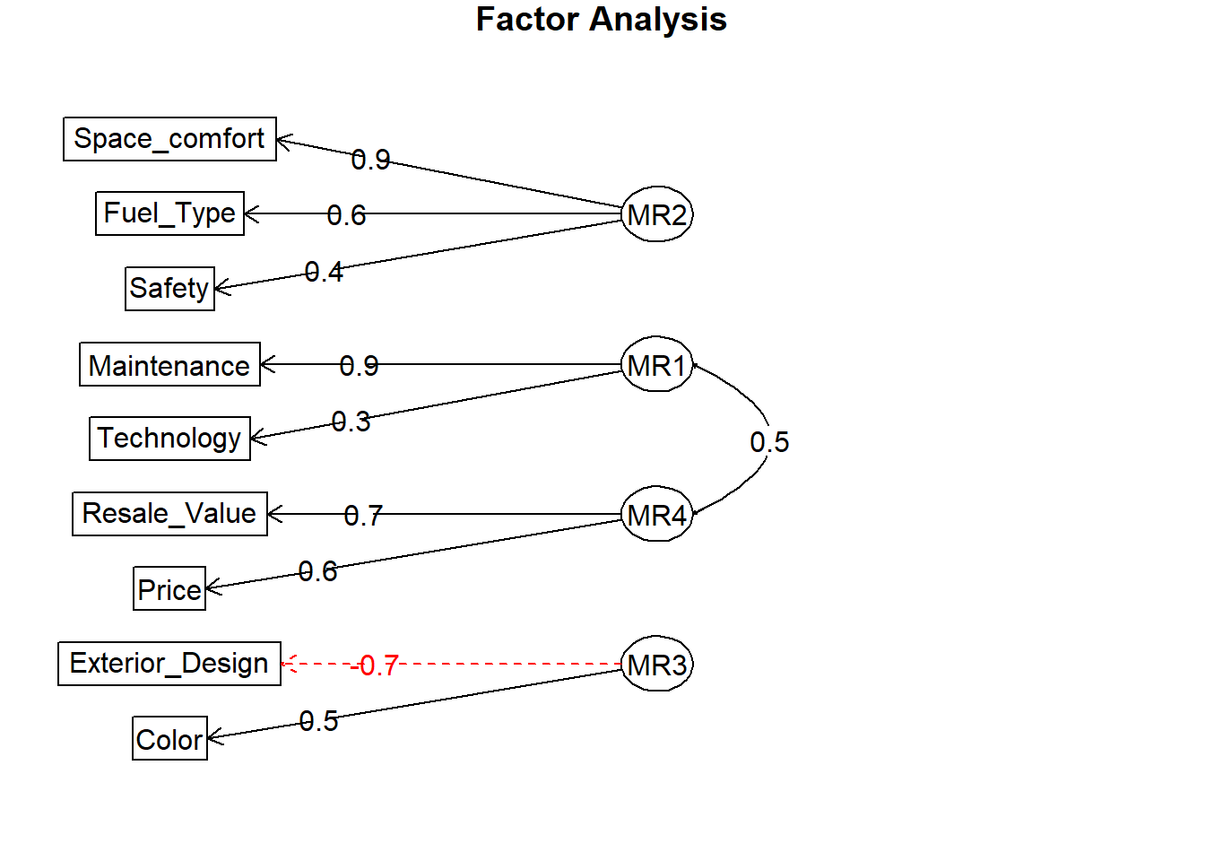
Adequacy Test
print(obli4factor)## Factor Analysis using method = minres
## Call: fa(r = data, nfactors = 4, rotate = "oblimin", fm = "minres")
## Standardized loadings (pattern matrix) based upon correlation matrix
## MR2 MR1 MR4 MR3 h2 u2 com
## Price 0.23 -0.02 0.60 0.01 0.37 0.63 1.3
## Safety 0.42 -0.26 -0.09 0.23 0.29 0.71 2.4
## Exterior_Design 0.03 0.02 0.00 -0.67 0.45 0.55 1.0
## Space_comfort 0.87 0.05 -0.02 -0.06 0.78 0.22 1.0
## Technology 0.28 0.34 -0.22 -0.02 0.19 0.81 2.7
## Resale_Value -0.12 0.11 0.69 0.00 0.61 0.39 1.1
## Fuel_Type 0.57 -0.03 0.11 0.02 0.31 0.69 1.1
## Color -0.05 0.29 0.01 0.48 0.37 0.63 1.7
## Maintenance 0.02 0.90 0.06 0.03 0.87 0.13 1.0
##
## MR2 MR1 MR4 MR3
## SS loadings 1.41 1.13 0.95 0.75
## Proportion Var 0.16 0.13 0.11 0.08
## Cumulative Var 0.16 0.28 0.39 0.47
## Proportion Explained 0.33 0.27 0.22 0.18
## Cumulative Proportion 0.33 0.60 0.82 1.00
##
## With factor correlations of
## MR2 MR1 MR4 MR3
## MR2 1.00 0.05 -0.13 -0.13
## MR1 0.05 1.00 0.55 0.17
## MR4 -0.13 0.55 1.00 -0.01
## MR3 -0.13 0.17 -0.01 1.00
##
## Mean item complexity = 1.5
## Test of the hypothesis that 4 factors are sufficient.
##
## The degrees of freedom for the null model are 36 and the objective function was 1.58 with Chi Square of 110.8
## The degrees of freedom for the model are 6 and the objective function was 0.03
##
## The root mean square of the residuals (RMSR) is 0.01
## The df corrected root mean square of the residuals is 0.04
##
## The harmonic number of observations is 75 with the empirical chi square 1.12 with prob < 0.98
## The total number of observations was 75 with Likelihood Chi Square = 2.07 with prob < 0.91
##
## Tucker Lewis Index of factoring reliability = 1.334
## RMSEA index = 0 and the 90 % confidence intervals are 0 0.057
## BIC = -23.83
## Fit based upon off diagonal values = 1
## Measures of factor score adequacy
## MR2 MR1 MR4 MR3
## Correlation of (regression) scores with factors 0.90 0.94 0.84 0.76
## Multiple R square of scores with factors 0.82 0.88 0.71 0.57
## Minimum correlation of possible factor scores 0.63 0.76 0.41 0.15The root mean square of residuals (RMSR) for the final four factor model is 0.01. This value should close to zero to have an acceptable model. Also, the Root Mean Square Error of Approximation (RMSEA) index is 0, and it shows a good model fit as it’s below 0.05. Finally, the Tucker-Lewis Index (TLI) is 1.334, which is also an acceptable value considering it’s over 0.9.
What are the factors?
Here, we have four factors. According to the grouping of the variables, we can name them as Technological benefits, Functional benefits, Aesthetics, and Economic value.
| Factor 1 | Factor 2 | Factor 3 | Factor 4 |
|---|---|---|---|
| Maintenance | Space comfort | Exterior design | Resale value |
| Technology | Fuel type | Color | Price |
| Safety | |||
| Technological benefits | Functional benefits | Aesthetics | Economic value |
factornal function for maximum likelihood factor analysis
The factanal( ) function produces maximum likelihood factor analysis for multivariate normal data. Since, the variables are on likert scale this method is not a good choice for this data set. If you want to apply maximum likelihood method for a data set first, test the multivariate normality of data using he following codes:
library(MVN)
mvn(data, univariateTest="SW",univariatePlot = "qqplot",multivariatePlot="qq",mvnTest="mardia")
Here, the “mardia” test is test is used to check the multivariate normality of data. Now, to apply Maximum Likelihood method to extract factors use the following codes:
fitmax=factanal(data,factors = 1,rotation = "varimax")```print(fitmax, digits=2, cutoff=.3, sort=TRUE)`
Start with factor one, and repeat until you get a significant number of factors. Then, you can plot the resulted solution using the following codes:
load <- fitmax$loadings[,1]
plot(load,type="n") # set up plot text(load,labels=names(data),cex=.7) # add variable names
violets are \(\color{blue}{\text{lovely blue}}\)
Further details:
1. https://rpubs.com/jeeva1407/367782
2. https://rpubs.com/aaronsc32/factor-analysis-introduction
3. https://rpubs.com/ykwon0407/89429
4. http://rpubs.com/nikkev/pca-factor 5. Applied Multivariate Statistical Analysis By R.A. Johnson & DW Wichern
Reading data in different formats:
http://www.sthda.com/english/wiki/reading-data-from-txt-csv-files-r-base-functions
Univariate and multivariate normality tests
https://rpubs.com/lozza44/263609
https://journal.r-project.org/archive/2014/RJ-2014-031/RJ-2014-031.pdf
http://www.biosoft.hacettepe.edu.tr/MVN/